r1,r2 = 425, 435
no_lead_files = ["processed_data/run408"] +  ["processed_data/run{}.csv".format(i) for i in range(r1,r2+1)]

r1,r2 = 410, 421
lead_files = ["processed_data/run{}".format(i) for i in range(r1,r2+1)] + ["processed_data/run422.csv"]
from MuDataFrame import *

mdfo_c = [] #collection of objects

for file in lead_files:
    mdfo_c.append(MuDataFrame(file)) #Muon Data Frame Object for Lead
mdfo_c
bdfo_c = [] #collection of objects

for file in no_lead_files:
    bdfo_c.append(MuDataFrame(file)) #Muon Data Frame Object for Lead
bdfo_c
Combining All Lead Brick and Non-Lead Brick Muon Data Frame Objects
import copy

mdf_list = [i.events_df for i in mdfo_c]
mdf_lead = mdfo_c[0].getMergedMDF(mdf_list)

mdfo_lead = copy.copy(mdfo_c[0])
mdfo_lead.events_df = mdf_lead
num_events_lead = len(mdf_lead.index)/(10**6) #Millions
num_events_lead
mdf_list = [i.events_df for i in bdfo_c]
mdf_calib = bdfo_c[0].getMergedMDF(mdf_list)

mdfo_calib = copy.copy(bdfo_c[0])
mdfo_calib.events_df = mdf_calib
num_events_calib = len(mdf_calib.index)/(10**6) #Millions
num_events_calib
We have 1.3 Million events with lead brick installation and 1.3 Million events with no lead bricks.
Fixing the Angle Calculation Issue
def fixedAnglesDf(df,dfo):
        df['theta_x1'] = dfo.events_df.eval("asymL2/asymL1") * (180 / np.pi)
        df['theta_y1'] = dfo.events_df.eval("asymL1/asymL2") * (180 / np.pi)
        df['theta_x2'] = dfo.events_df.eval("asymL4/asymL3") * (180 / np.pi)
        df['theta_y2'] = dfo.events_df.eval("asymL3/asymL4") * (180 / np.pi)
        # process Z
        asymT1 = df['asymL1'].values
        asymT2 = df['asymL2'].values
        asymT3 = df['asymL3'].values
        asymT4 = df['asymL4'].values
        zangles = np.arctan(
            np.sqrt((asymT1 - asymT3)**2 +
                    (asymT2 - asymT4)**2) / dfo.d_asym) * (180 / np.pi)
        df["z_angle"] = zangles
        return df
#calibration
mdfo_calib.events_df = fixedAnglesDf(mdfo_calib.events_df,mdfo_calib)

#leadbricks
mdfo_lead.events_df = fixedAnglesDf(mdfo_lead.events_df,mdfo_lead)
Changin event times to serial time
from datetime import datetime, timedelta
times_lead =  np.array([datetime.strptime(date, '%Y-%m-%d %H:%M:%S.%f') for date in mdfo_lead.events_df["event_time"].values])
from datetime import datetime, timedelta
times_calib436 =  np.array([datetime.strptime(date, '%Y-%m-%d %H:%M:%S.%f') for date in mdfoc_436.events_df["event_time"].values])
times_calib = np.array([datetime.strptime(date, '%Y-%m-%d %H:%M:%S.%f') for date in mdfo_calib.events_df["event_time"].values])
times_l436 = [mdfo_calib.get("event_time")[-1]]

for i in range(1,len(times_calib436)):
    del_t = times_calib436[i] - times_calib436[i-1]
    times_l436.append(del_t.microseconds+ times_l436[i-1])
times_l1 = [0]
times_l2 = [0]

for i in range(1,len(times_lead)):
    del_t = times_lead[i] - times_lead[i-1]
    times_l1.append(del_t.microseconds + times_l1[i-1])

for i in range(1,len(times_calib)):
    del_t = times_calib[i] - times_calib[i-1]
    times_l2.append(del_t.microseconds+ times_l2[i-1])
mdfo_lead.events_df["event_time"] = times_l1
mdfo_calib.events_df["event_time"] = times_l2
mdfoc_436.events_df["event_time"] = times_l436
mdfo_calib.show()
toDays = 0.00000000001157407
duration_lead = (mdfo_lead.get("event_time")[-1] - mdfo_lead.get("event_time")[0])*toDays
duration_calib = (mdfo_calib.get("event_time")[-1] - mdfo_calib.get("event_time")[0])*toDays
duration_lead, duration_calib
The lead experiment lasted 4.80409327312524 days while calibration experiment has taken 4.132068114122623 days so far.
mu_rate_lead = num_events_lead / duration_lead #million per day
mu_rate_lead
mu_rate_calib = num_events_calib / duration_calib #million per day
mu_rate_calib
The muon rate for with bricks is $0.271$ Million Events per day, while without is $0.272$ Million Events per day.
Tomogram Generation
Testing of new equations.
Zplane of T1 and T2 are defined to be $0$ while that of T3 and T4 are defined to be $-d_{sep}$. Zplane of bricks are $d_{brick}$.
def getPhysicalUnits(asym):
    return (55 / 0.6) * asym

def getXatZPlane(x1,x2,zplane,dsep):
    x = (zplane/dsep)*(getPhysicalUnits(x1)-getPhysicalUnits(x2))+getPhysicalUnits(x1)
    return x
import scipy.interpolate, scipy.optimize

def getLeadDistanceinXArr(xx_lead,xx_calib,bins):
    b1 = plt.hist(xx_lead,bins=bins,density=True,range=(-50,50))
    b2 = plt.hist(xx_calib,bins=bins,density=True,range=(-50,50))
    x  = np.array([i*5 for i in range(1,12)])
    y1 = [1 for i in range(len(x))]
    y2 = b1[0]/b2[0]
    interp1 = scipy.interpolate.InterpolatedUnivariateSpline(x, y1)
    interp2 = scipy.interpolate.InterpolatedUnivariateSpline(x, y2)
    new_x = np.linspace(x.min(), x.max(), 100)
    new_y1 = interp1(new_x)
    new_y2 = interp2(new_x)
    idx = np.argwhere(np.diff(np.sign(new_y1 - new_y2)) != 0)

    plt.plot(x, y1, marker='o', mec='none', ms=4, lw=1, label='y1')
    plt.plot(x, y2, marker='o', mec='none', ms=4, lw=1, label='y2')
    plt.plot(new_x[idx], new_y1[idx], 'ro', ms=7, label='intersection')
    plt.legend(frameon=False, fontsize=10, numpoints=1, loc='lower left')
    plt.ylim(0.7,1.05)
    plt.xlim(0,60)
    plt.show()
    return list(new_x[idx])
def testTomogram(mdfo_lead,mdfo_calib,bins):
xx_lead = mdfo_lead.get("xx")
yy_lead = mdfo_lead.get("yy")
xx_calib = mdfo_calib.get("xx")
yy_calib = mdfo_calib.get("yy")
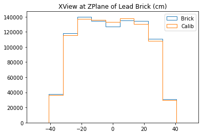
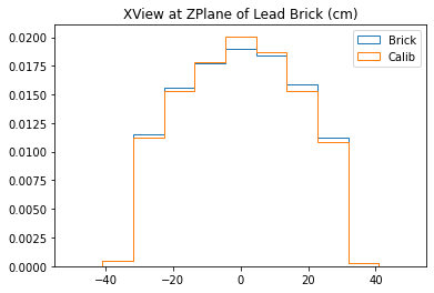
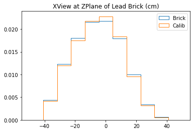
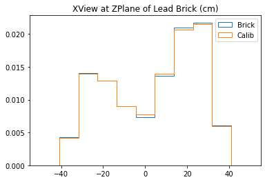
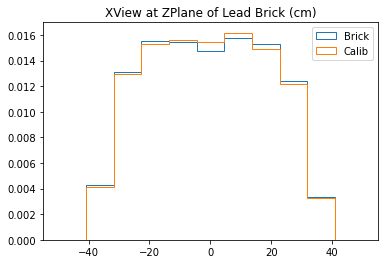
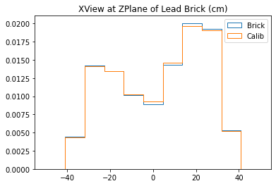
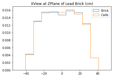
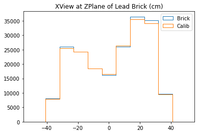
b1 =plt.hist(xx_lead,bins=bins,alpha=1,label="Brick",density=True,range=(-50,50),histtype='step')
b2 =plt.hist(xx_calib,bins=bins,alpha=1,label="Calib",density=True,range=(-50,50),histtype='step')
plt.title("XView at ZPlane of Lead Brick (cm)")
plt.legend()
plt.show()
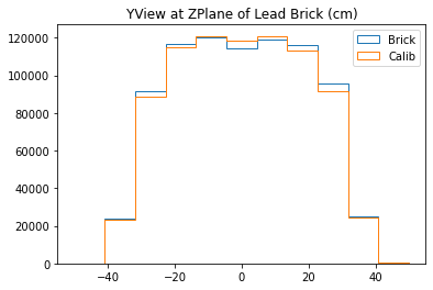
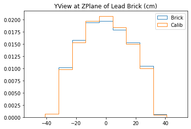
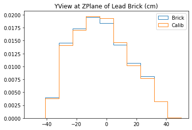
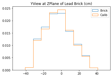
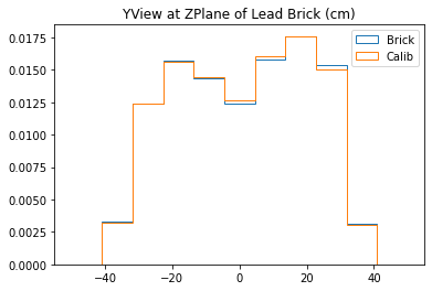
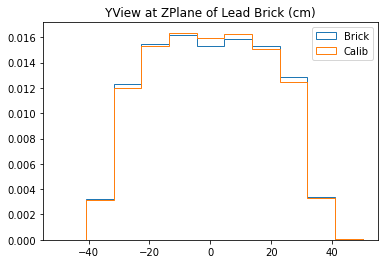
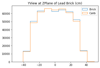
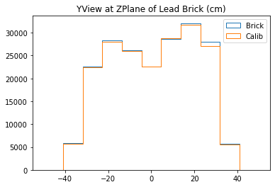
b3 =plt.hist(yy_lead,bins=bins,alpha=1,label="Brick",density=True,range=(-50,50),histtype='step')
b4 =plt.hist(yy_calib,bins=bins,alpha=1,label="Calib",density=True,range=(-50,50),histtype='step')
plt.title("YView at ZPlane of Lead Brick (cm)")
plt.legend()
plt.show()
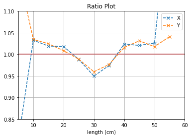
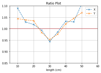
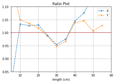
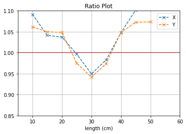
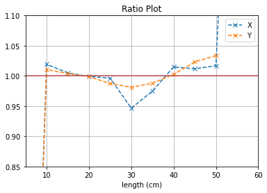
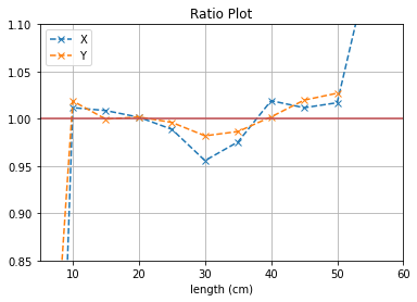
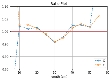
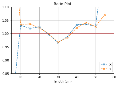
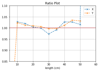
plt.plot([i*5 for i in range(1,12)], (b1[0]/b2[0]),'--x',label = "X")
plt.plot([i*5 for i in range(1,12)], (b3[0]/b4[0]),'--x',label = "Y")
plt.axhline(y=1, color='r')
plt.title("Ratio Plot")
plt.xlabel("length (cm)")
plt.grid()
plt.legend()
plt.ylim(0.85,1.1)
plt.xlim(5,60)
plt.show()
#x_dist = getLeadDistanceinXArr(xx_lead,xx_calib,bins=11)
#y_dist = getLeadDistanceinXArr(yy_lead,yy_calib,bins=11)
#return x_dist,y_dist
def testTomogramRaw(mdfo_lead,mdfo_calib,bins):
xx_lead = mdfo_lead.get("xx")
yy_lead = mdfo_lead.get("yy")
xx_calib = mdfo_calib.get("xx")
yy_calib = mdfo_calib.get("yy")
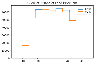
b1 =plt.hist(xx_lead,bins=bins,alpha=1,label="Brick",range=(-50,50),histtype='step')
b2 =plt.hist(xx_calib,bins=bins,alpha=1,label="Calib",range=(-50,50),histtype='step')
plt.title("XView at ZPlane of Lead Brick (cm)")
plt.legend()
plt.show()
b3 =plt.hist(yy_lead,bins=bins,alpha=1,label="Brick",range=(-50,50),histtype='step')
b4 =plt.hist(yy_calib,bins=bins,alpha=1,label="Calib",range=(-50,50),histtype='step')
plt.title("YView at ZPlane of Lead Brick (cm)")
plt.legend()
plt.show()
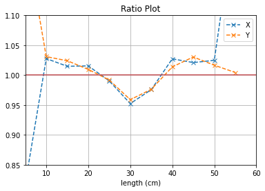
plt.plot([i*5 for i in range(1,12)], (b1[0]/b2[0]),'--x',label = "X")
plt.plot([i*5 for i in range(1,12)], (b3[0]/b4[0]),'--x',label = "Y")
plt.axhline(y=1, color='r')
plt.title("Ratio Plot")
plt.xlabel("length (cm)")
plt.grid()
plt.legend()
plt.ylim(0.85,1.1)
plt.xlim(5,60)
plt.show()
#x_dist = getLeadDistanceinXArr(xx_lead,xx_calib,bins=11)
#y_dist = getLeadDistanceinXArr(yy_lead,yy_calib,bins=11)
#return x_dist,y_dist
Test Code
xx_lead = getXatZPlane(mdfo_lead.get("asymL1"),mdfo_lead.get("asymL3"),42,165)
yy_lead = getXatZPlane(mdfo_lead.get("asymL2"),mdfo_lead.get("asymL4"),42,165)
xx_calib = getXatZPlane(mdfo_calib.get("asymL1"),mdfo_calib.get("asymL3"),42,165)
yy_calib = getXatZPlane(mdfo_calib.get("asymL2"),mdfo_calib.get("asymL4"),42,165)
b1 =plt.hist(xx_lead,bins=11,alpha=1,label="Brick",density=True,range=(-50,50),histtype='step')
b2 =plt.hist(xx_calib,bins=11,alpha=1,label="Calib",density=True,range=(-50,50),histtype='step')
plt.title("XView ZPlane of Lead Brick (cm)")
plt.legend()
plt.show()
b3 = plt.hist(yy_lead,bins=11,alpha=1,label="Brick",density=True,range=(-50,50),histtype='step')
b4 = plt.hist(yy_calib,bins=11,alpha=1,label="Calib",density=True,range=(-50,50),histtype='step')
plt.title("YView ZPlane of Lead Brick (cm)")
plt.legend()
plt.show()
plt.plot([i*5 for i in range(1,12)], (b1[0]/b2[0]),'--x')
plt.axhline(y=1, color='r')
plt.title("X View Ratio")
plt.xlabel("length (cm)")
plt.grid()
plt.show()
plt.plot([i*5 for i in range(1,12)], (b3[0]/b4[0]),'--x')
plt.axhline(y=1, color='r')
plt.title("Y View Ratio")
plt.xlabel("length (cm)")
plt.grid()
plt.show()
import scipy.interpolate, scipy.optimize

def getLeadDistanceinXArr(xx_lead,xx_calib,bins):
    b1 = plt.hist(xx_lead,bins=bins,density=True,range=(-50,50))
    b2 = plt.hist(xx_calib,bins=bins,density=True,range=(-50,50))
    x  = np.array([i*5 for i in range(1,12)])
    y1 = [1 for i in range(len(x))]
    y2 = b1[0]/b2[0]
    interp1 = scipy.interpolate.InterpolatedUnivariateSpline(x, y1)
    interp2 = scipy.interpolate.InterpolatedUnivariateSpline(x, y2)
    new_x = np.linspace(x.min(), x.max(), 100)
    new_y1 = interp1(new_x)
    new_y2 = interp2(new_x)
    idx = np.argwhere(np.diff(np.sign(new_y1 - new_y2)) != 0)

    plt.plot(x, y1, marker='o', mec='none', ms=4, lw=1, label='y1')
    plt.plot(x, y2, marker='o', mec='none', ms=4, lw=1, label='y2')
    plt.plot(new_x[idx], new_y1[idx], 'ro', ms=7, label='intersection')
    plt.legend(frameon=False, fontsize=10, numpoints=1, loc='lower left')
    plt.ylim(0.5,1.3)
    plt.xlim(0,60)
    plt.show()
    return list(new_x[idx])
x_dist = getLeadDistanceinXArr(xx_lead,xx_calib,bins=11)
x_dist = x_dist[2] - x_dist[1]
x_dist
y_dist = getLeadDistanceinXArr(yy_lead,yy_calib,bins=11)
y_dist = y_dist[1] - y_dist[0]
y_dist
Testing Tomogram
x_dist,y_dist = testTomogram(mdfo_lead,mdfo_calib,bins=11)
mdfo_lead.keep4by4Events()
mdfo_calib.keep4by4Events()

testTomogram(mdfo_lead,mdfo_calib,bins=11)
x_dist = x_dist[2] - x_dist[1]
y_dist = y_dist[1] - y_dist[0]
x_dist,y_dist
Tomogram Generation Test Code
xx_lead = getXatZPlane(mdfo_lead.get("asymL1"), mdfo_lead.get("asymL3"), 42,
                       165)
yy_lead = getXatZPlane(mdfo_lead.get("asymL2"), mdfo_lead.get("asymL4"), 42,
                       165)
xx_calib = getXatZPlane(mdfo_calib.get("asymL1"), mdfo_calib.get("asymL3"), 42,
                        165)
yy_calib = getXatZPlane(mdfo_calib.get("asymL2"), mdfo_calib.get("asymL4"), 42,
                        165)
xx_calib436 = getXatZPlane(mdfoc_436.get("asymL1"), mdfoc_436.get("asymL3"), 42,
                        165)
yy_calib436 = getXatZPlane(mdfoc_436.get("asymL2"), mdfoc_436.get("asymL4"), 42,
                        165)
mdfoc_436.events_df["xx"] = xx_calib436
mdfoc_436.events_df["yy"] = yy_calib436
mdfo_lead.events_df["xx"] = xx_lead
mdfo_lead.events_df["yy"] = yy_lead

mdfo_calib.events_df["xx"] = xx_calib
mdfo_calib.events_df["yy"] = yy_calib
num_lead_events = len(mdfo_lead.events_df.index)
lead_events_seq = [i for i in range(num_lead_events)]

num_calib_events = len(mdfo_calib.events_df.index)
calib_events_seq = [i for i in range(num_calib_events)]
ev436 = len(mdfoc_436.events_df.index)
num_calib_events436 = ev436 + num_calib_events
calib_events_seq436 = [i for i in range(num_calib_events, num_calib_events436)]
mdfoc_436.events_df["event_num"] = calib_events_seq436
mdfo_lead.events_df["event_num"] = lead_events_seq
mdfo_calib.events_df["event_num"] = calib_events_seq
mdfo_calib.show()
import copy

mdf_calib = mdfo_calib.events_df
mdf_lead = mdfo_lead.events_df

mdfo_calib.og_df = mdf_calib.copy()
mdfo_lead.og_df = mdf_lead.copy()
Create combined emission files
mdf_lead.to_csv("processed_data/lead_data.csv")
mdf_calib.to_csv("processed_data/calibration_data.csv")
Loading Muon DataFrame Aggregate Data Files
import copy
from MuDataFrame import MuDataFrame

mdfo_calib = MuDataFrame("processed_data/calib_data.csv")
mdfo_lead = MuDataFrame("processed_data/lead_data.csv")

mdfo_calib.events_df.drop(columns=["Unnamed: 0","index"],axis=1, inplace=True)
mdfo_lead.events_df.drop(columns=["Unnamed: 0","index"],axis=1, inplace=True)

mdf_calib = mdfo_calib.events_df
mdf_lead = mdfo_lead.events_df

mdfo_calib.og_df = mdf_calib.copy()
mdfo_lead.og_df = mdf_lead.copy()
mdfo_calib.show()
mdfo_lead.show()
import copy

mdf_list = [mdfo_calib.events_df, mdfoc_436.events_df]
mdf_calib = mdfo_calib.getMergedMDF(mdf_list)

mdfo_calib = copy.copy(mdfo_calib)
mdfo_calib.events_df = mdf_calib
mdf_calib.to_csv("processed_data/calib_data.csv")
test 2
bins = 11
b1 = plt.hist(xx_lead, bins=bins, alpha=1, label="Brick",
              density=True, range=(-50, 50), histtype='step')
b2 = plt.hist(xx_calib, bins=bins, alpha=1, label="Calib",
              density=True, range=(-50, 50), histtype='step')
plt.title("XView ZPlane of Lead Brick (cm)")
plt.legend()
plt.show()
b3 = plt.hist(yy_lead, bins=bins, alpha=1, label="Brick",
              density=True, range=(-50, 50), histtype='step')
b4 = plt.hist(yy_calib, bins=bins, alpha=1, label="Calib",
              density=True, range=(-50, 50), histtype='step')
plt.title("YView ZPlane of Lead Brick (cm)")
plt.legend()
plt.show()
mdf_lead_tomo = pd.DataFrame(list(zip(xx_lead,yy_lead)),columns=["xx","yy"])
mdf_calib_tomo = pd.DataFrame(list(zip(xx_calib,yy_calib)),columns=["xx","yy"])
mdf_lead_tomo
import plotly.express as px

bins = 20
fig = px.density_heatmap(mdf_lead_tomo, x="xx", y="yy", nbinsx=bins, nbinsy=bins, marginal_x="histogram", marginal_y="histogram", histnorm='probability')
fig.show()
import plotly.graph_objects as go
import plotly.express as px

fig = go.Figure(go.Histogram2d(x=mdf_lead_tomo.xx.values, y=mdf_lead_tomo.yy.values, coloraxis = "coloraxis"))
fig.update_layout(coloraxis = {'colorscale':'viridis'})
fig.show()
fig = px.density_heatmap(mdf_lead_tomo, x="xx", y="yy", nbinsx=bins, nbinsy=bins, marginal_x="histogram", marginal_y="histogram")
fig.show()
fig = px.density_heatmap(mdf_calib_tomo, x="xx", y="yy", nbinsx=bins, nbinsy=bins, marginal_x="histogram", marginal_y="histogram")
fig.show()
TO DO LIST:
- implement code to test out cut effects on tomogram quick (plotly 2D)
- Xview Yview comparisons
- figure out physics based cuts to generate tomogram
- add tomogram creation using diff and discrete
Interactive Analysis
mdfo_lead.reload()
mdfo_lead.keep4by4Events()
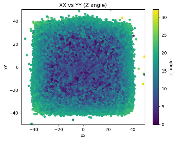
mdfo_lead.get3DScatterPlot(["xx","yy","z_angle"],"XX vs YY (Z angle)",(-50,50),(-50,50))
mdfo_lead.reload()
mdfo_lead.keep4by4Events()
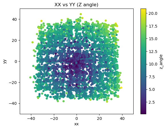
mdfo_lead.keepEvents("SmallCounter",120,">=")
mdfo_lead.get3DScatterPlot(["xx","yy","z_angle"],"XX vs YY (Z angle)",(-50,50),(-50,50))
light leak proof?
Idea of Small counters on top and also bottom of lead brick
bins = 11
xybins = np.linspace(-40,40,bins)
labels = [i for i in range(1,bins+1)]
labels =[1,2,3,4]
df1['binned'] = pd.cut(df1['Score'], bins,labels=labels)
print(df1)
import plotly.express as px

def doTomography(bins, mdf, title):
    fig = px.density_heatmap(mdf, x="xx", y="yy", title=title, nbinsx=bins, nbinsy=bins,
                             marginal_x="histogram", marginal_y="histogram")

    fig.update_layout(
    xaxis_title="XView (cm)",
    yaxis_title="YView (cm)",
    )
    fig.show()
%matplotlib inline
mdfo_lead.reload()
mdfo_calib.reload()
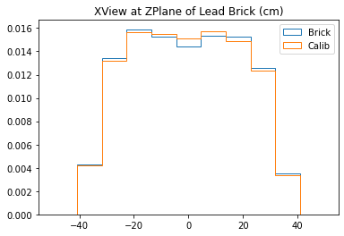
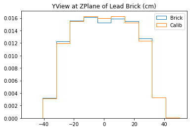
testTomogram(mdfo_lead,mdfo_calib,bins=11)
#doTomography(22, mdfo_lead.events_df, "Lead Bricks")
testTomogramRaw(mdfo_lead,mdfo_calib,bins=11)
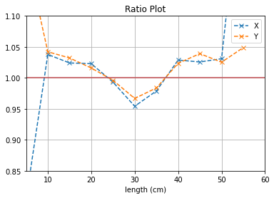
With no cuts made, we get the following dimensions:
Y(22.3,38.1) = 15.8 cm
X(23.1,37.7) = 14.6 cm
Testing Muons within 5 to 10 degree zenith angles
mdfo_lead.reload()
mdfo_calib.reload()

mdfo_lead.keep4by4Events()
mdfo_lead.keepEvents("z_angle",5,">=")
mdfo_lead.keepEvents("z_angle",10,"<=")

mdfo_calib.keep4by4Events()
mdfo_calib.keepEvents("z_angle",5,">=")
mdfo_calib.keepEvents("z_angle",10,"<=")

testTomogram(mdfo_lead,mdfo_calib,bins=11)
#doTomography(22, mdfo_lead.events_df, "Lead Bricks")
#doTomography(22, mdfo_calib.events_df, "No Lead Bricks")
Testing Faster Muons
Assuming faster muons are muons with low Sum TDCs. We will make a cut of less than equal to the mean.
mdfo_lead.reload()
mdfo_lead.keep4by4Events()
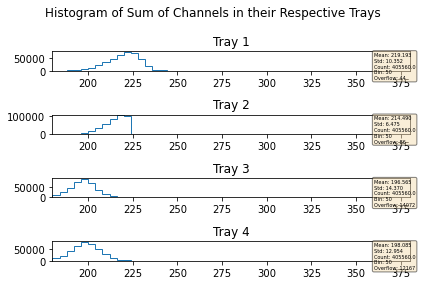
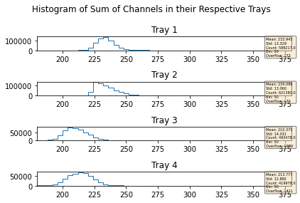
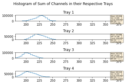
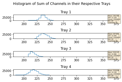
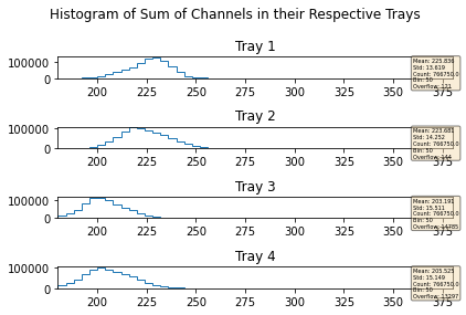
mdfo_lead.getChannelSumPlots()

mdfo_calib.reload()
mdfo_calib.keep4by4Events()

mdfo_calib.getChannelSumPlots()

mdfo_lead.keepEvents("sumL2",223,"<=")
mdfo_lead.getChannelSumPlots()
mdfo_calib.keepEvents("sumL2",223,"<=")
mdfo_calib.getChannelSumPlots()

mdfo_lead.reload()
mdfo_calib.reload()

mdfo_lead.keep4by4Events()
mdfo_lead.keepEvents("sumL2",223,"<=")


mdfo_calib.keep4by4Events()
mdfo_calib.keepEvents("sumL2",223,"<=")

testTomogram(mdfo_lead,mdfo_calib,bins=11)
#doTomography(22, mdfo_lead.events_df, "Lead Bricks")
Limiting to straight muons.
mdfo_lead.reload()
mdfo_calib.reload()

mdfo_lead.keep4by4Events()
mdfo_lead.keepEvents("sumL2",223,"<=")
mdfo_lead.keepEvents("z_angle",5,">=")
mdfo_lead.keepEvents("z_angle",10,"<=")

mdfo_calib.keep4by4Events()
mdfo_calib.keepEvents("sumL2",223,"<=")
mdfo_calib.keepEvents("z_angle",5,">=")
mdfo_calib.keepEvents("z_angle",10,"<=")

testTomogram(mdfo_lead,mdfo_calib,bins=11)
#doTomography(22, mdfo_lead.events_df, "Lead Bricks")
The dimensions appear to be shorter than actual
Testing Slower Muons
Assuming slower muons are muons with high Sum TDCs. We will make a cut of greater than equal to the mean.
mdfo_lead.reload()
mdfo_lead.keepEvents("sumL2",223,">=")
mdfo_lead.getChannelSumPlots()

mdfo_calib.reload()
mdfo_calib.keepEvents("sumL2",223,">=")
mdfo_calib.getChannelSumPlots()
%matplotlib inline
mdfo_lead.reload()
mdfo_calib.reload()
mdfo_lead.keep4by4Events()
mdfo_lead.keepEvents("sumL2",223,">=")
mdfo_calib.keep4by4Events()
mdfo_calib.keepEvents("sumL2",223,">=")
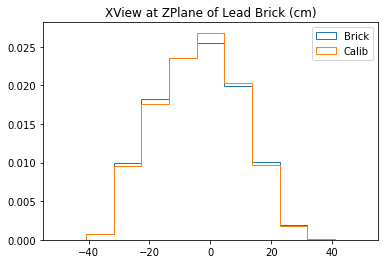
testTomogram(mdfo_lead,mdfo_calib,bins=11)
#doTomography(22, mdfo_lead.events_df, "Lead Bricks")

X View: 19.8 cm
Y View: 18.8 cm
The results with slow muons are much better which are expected since more of such classes of muons have not passed through the lead bricks.
Same Analysis but now with time restrictions
Keeping all data that is within 4 days of operation.
mdfo_lead.reload()
mdfo_calib.reload()
fourDays = 345600000000 #microseconds
mdfo_lead.reload()
mdfo_calib.reload()

mdfo_lead.keepEvents("event_time",fourDays,"<=")
mdfo_lead.keep4by4Events()

mdfo_calib.keepEvents("event_time",fourDays,"<=")
mdfo_calib.keep4by4Events()

testTomogram(mdfo_lead,mdfo_calib,bins=11)

Keeping Slower Muons
mdfo_lead.reload()
mdfo_calib.reload()

mdfo_lead.keep4by4Events()
mdfo_lead.keepEvents("event_time",fourDays,"<=")
mdfo_lead.getChannelSumPlots()
mdfo_lead.keepEvents("event_time",fourDays,"<=")
mdfo_lead.keepEvents("sumL2",223,">=")
mdfo_lead.keepEvents("sumL3",210,">=")
mdfo_lead.getChannelSumPlots()
mdfo_lead.reload()
mdfo_calib.reload()

mdfo_lead.keep4by4Events()
mdfo_lead.keepEvents("event_time",fourDays,"<=")
mdfo_lead.keepEvents("sumL2",220,">=")

mdfo_calib.keep4by4Events()
mdfo_calib.keepEvents("event_time",fourDays,"<=")
mdfo_calib.keepEvents("sumL2",220,">=")


testTomogram(mdfo_lead,mdfo_calib,bins=11)
The length seems to be extracted pretty well.
Analysis with same Muon numbers
Seeing the number of 4 by 4 muons.
mdfo_lead.reload()
mdfo_lead.keep4by4Events()
m1 = mdfo_lead.events_df
ms1 = len(m1.index)
ms1
mdfo_calib.reload()
mdfo_calib.keep4by4Events()
m2 = mdfo_calib.events_df
ms2 = len(m2.index)
ms2
muon_num = min(ms2,ms1)
muon_num
Density Plot
mdfo_lead.reload()
mdfo_calib.reload()

mdfo_lead.keep4by4Events()
mdfo_lead.keepEvents("event_num",muon_num,"<=")

mdfo_calib.keep4by4Events()
mdfo_calib.keepEvents("event_num",muon_num,"<=")

testTomogram(mdfo_lead,mdfo_calib,bins=11)
Actual Numbers
testTomogramRaw(mdfo_lead,mdfo_calib,bins=11)
Actual Numbers for slow muons analysis
mdfo_lead.reload()
mdfo_lead.keep4by4Events()
mdfo_lead.getChannelSumPlots()
tdc_thresh = 220

mdfo_lead.reload()
mdfo_lead.keep4by4Events()
mdfo_lead.keepEvents("sumL1",tdc_thresh,">=")


m1 = mdfo_lead.events_df
ms1 = len(m1.index)
ms1
mdfo_calib.reload()
mdfo_calib.keep4by4Events()
mdfo_calib.keepEvents("sumL1",tdc_thresh,">=")


m2 = mdfo_calib.events_df
ms2 = len(m2.index)
ms2
muon_num = min(ms2,ms1)
muon_num
mdfo_lead.reload()
mdfo_calib.reload()

mdfo_lead.keep4by4Events()
mdfo_lead.keepEvents("sumL2",tdc_thresh,">=")
mdfo_lead.keepEvents("event_num",muon_num,"<=")

mdfo_calib.keep4by4Events()
mdfo_calib.keepEvents("sumL2",tdc_thresh,">=")
mdfo_calib.keepEvents("event_num",muon_num,"<=")

testTomogramRaw(mdfo_lead,mdfo_calib,bins=11)
Full Data Set Comparison
As of 02/32/20 , we have 1.3 Mill $\mu$ events for both lead brick and no lead brick runs.
One observation was that we see more muon events radially away from the region of lead bricks in the X-Y plane. This is predicted since we expect some scattered muon events from the lead bricks to still trigger the system. This may be useful information because we can calculate the angle associated with the effect of the scattering and use that in tomography as well.
Plans moving forward
Main Plan
- Clean report ready with 2D histo + resolution val
- Linking TDC info for tomo
- correct existing
- get ortho coordinate and generate tomo
- tomogram generation through diffTDC data
- associate muon speed to each event and use this info for tomography
- generate muon speed dist from data set
- Cuts on temporal space
Later
- RL work with Cris
- tomogram using discrete angle binned data
- study of factors affecting tomogram generation
- tomogram visualization
- ML applications
- Resolution determination
- Better Muon Track Reco algorithms