PHYS 540 Presentation
Quantum Wells and Transmission
Sadman Ahmed Shanto
One Dimensional Quantum Well

- A quantum well is a potential well with only discrete energy values.
- They have applications in lasers, photodetectors, modulators, switches, semiconductors, junctions...
Example Structure: GaAs - AlGaAs
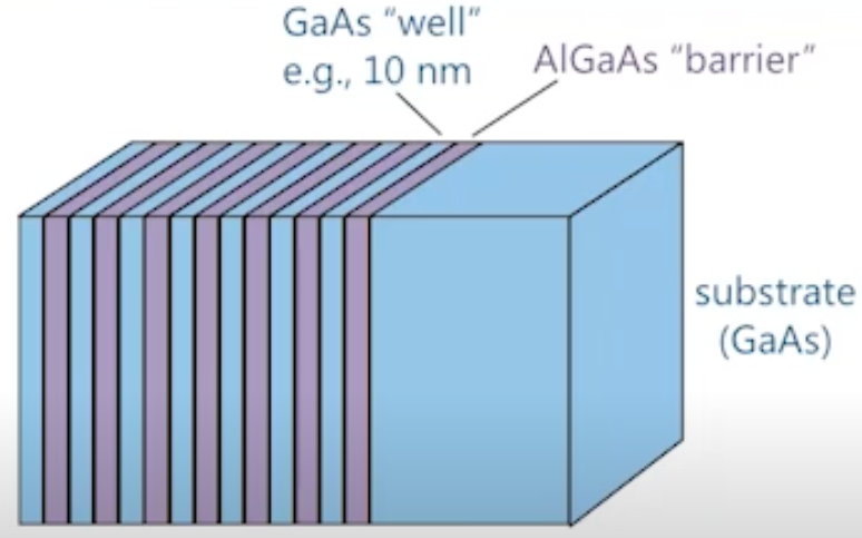
- Electrons see lower energies in the well
- This leads to "particle in a box" phenomena (quantum confinement in 1D)
Solving the 1D Quantum Well
- Assume Quantum Wells are along $\hat z$
- quantum confinement is thus also along $\hat z$ (potential width comparable to de Brogile wavelength of electrons)
- electrons free to move in $\hat x, \hat y$ (i.e. free plane waves)
Solving the 1D Quantum Well
$$ -\frac{h^2}{2 m_{e f f}} \nabla^2 \psi(\mathbf{r})+V(z) \psi(\mathbf{r})=E \psi(\mathbf{r}) $$
$$ \Rightarrow -\frac{h^2}{2 m_{eff}} \nabla_{xy}^2 \psi(\mathrm{r})-\frac{h^2}{2 m_{e f f}} \frac{\partial^2}{\partial z^2} \psi(\mathrm{r})+V(z) \psi(\mathrm{r})=E \psi(\mathrm{r})$$
where $\nabla_{x y}^2 \equiv \frac{\partial^2}{\partial x^2}+\frac{\partial^2}{\partial y^2}$
We postulate a separation $$ \psi(\mathbf{r})=\psi_n(z) \psi_{x y}\left(r_{xy}\right) $$
Substituting this $\psi(\mathbf{r})=\psi_n(z) \psi_{x y}\left(\mathrm{r}_{x y}\right)$ into the Schrödinger equation
$$-\frac{h^2}{2 m_{\text {eff }}} \nabla_{xy}^2 \psi(\mathbf{r})-\frac{h^2}{2 m_{\text {eff }}} \frac{\partial^2}{\partial z^2} \psi(\mathbf{r})+V(z) \psi(\mathbf{r})=E \psi(\mathbf{r})$$
and dividing this by $\psi(\mathbf{r})$, we get
$$-\frac{h^2}{2 m_{eff}} \frac{1}{\psi_{xy}\left(r_{xy}\right)} \nabla_{xy}^2 \psi_{xy}\left(r_{xy}\right)-\frac{h^2}{2 m_{eff}} \frac{1}{\psi_n(z)} \frac{\partial^2}{\partial z^2} \psi_n(z)+V(z)=E$$
We can separate the equation to get
$$\text{LHS:} -\frac{h^2}{2 m_{eff}} \nabla_{xy}^2 \psi_{xy} (r_{xy}) = E_{xy} \psi_{xy} (r_{xy}) $$
with $E_{x y} = \frac{\hbar^2 k_{xy}^2}{2 m_{eff}}$
Plane wave solutions in $\hat x, \hat y$
$$\large\psi_{xy} (r_{xy}) \propto e^{(i k_{xy} . r_{xy})} $$
$$\text{RHS:} -\frac{h^2}{2 m_{e f f}} \frac{d^2}{d z^2} \psi_n(z)+V(z) \psi_n(z)=E_n \psi_n(z)$$
with $E_n=E-E_{x y}$ and $E_{x y} = \frac{\hbar^2 k_{xy}^2}{2 m_{eff}}$
We solve this numerically - just like we did a few weeks back in our homework
$$ \tiny \hat H = \begin{pmatrix} -2 (-\frac{\hbar^2}{2 m \Delta^2}) + V_0 & -\frac{\hbar^2}{2 m \Delta^2} & 0 & & \\ -\frac{\hbar^2}{2 m \Delta^2} & -2 (-\frac{\hbar^2}{2 m \Delta^2}) + V_1 & -\frac{\hbar^2}{2 m \Delta^2} & & \\ 0 & -\frac{\hbar^2}{2 m \Delta^2} & -2(-\frac{\hbar^2}{2 m \Delta^2}) + V_2 & & \\ & & &\ddots & \\ &&&&-2(-\frac{\hbar^2}{2 m \Delta^2}) + V_{N-1}\end{pmatrix} $$
Using this expression, is now easy to write a numerical form for $\hat H$ for any potential term $V$ and use the magic of computers to diagonalize the matrix and obtain eigenvalues and eigenfunctions.
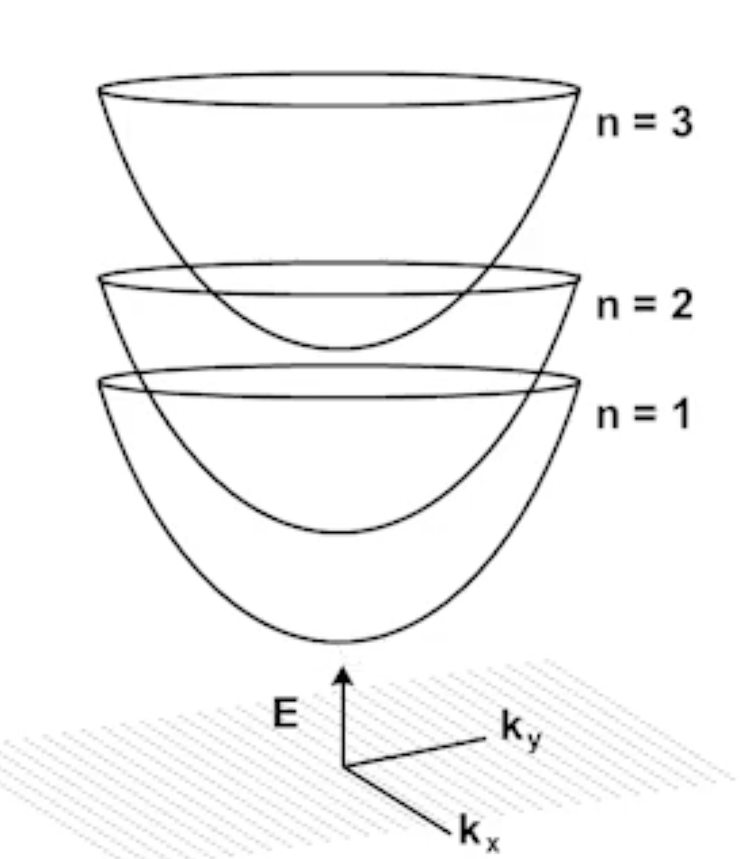
Subband Formations:
The total energies allowed are:
$$E = E_n + E_{xy}$$
Double Square Well Potential and an example - Ammonia Maser

The nitrogen in the NH$_3$ molecule has two degrees of freedom - it can oscillate up and down.
Consider starting from an initial state, where the nitrogen is localized on the left quantum well. The wavefunction can be formulated as a combination of the two lowest quantum states.
$$ |\psi(t=0)> = \frac{1}{\sqrt{2}}[|\psi_1>+|\psi_2>]$$
The time-resolved state is written as:
$$ |\psi(t)> = \frac{1}{\sqrt{2}}\left[e^{-iE_1t/\hbar}|\psi_1> +e^{-iE_2t/\hbar}|\psi_2> \right]$$
$$ = \frac{1}{\sqrt{2}}e^{-i(E_1 + E_2)t/(2\hbar)} \left[e^{i\Omega t/2}|\psi_1> + e^{-i\Omega t/2}|\psi_2> \right]$$
where the $\Omega$ is defined as:
$$\Omega = \frac{E_2- E_1}{\hbar}$$
Therefore, the probability density is given as:
$$ |\psi(x,t)|^2 = \frac{1}{2}(\psi_1^2+\psi_2^2) + cos(\Omega t)\psi_1\psi_2$$
At $t=\frac{\pi}{\Omega}$, the wavefunction becomes localized in the right quantum well.
$$ |\psi(x, t=\frac{\pi}{\Omega})|^2 = \frac{1}{2}|\psi_1 - \psi_2|^2$$
In this model, the nitrogen moves from left well to right well and back again with a frequency $f = \frac{\Omega}{2\pi}$.
The energy difference $E_1 - E_2$ is very small, which leads to a small frequency of the nitrogen inversion.
$\therefore$ The NH$_3$ molecule emits radiation through this process (i.e. acts as a Maser)
%matplotlib widget

from numpy import linspace, sqrt, ones, arange, diag, argsort, zeros
from scipy.linalg import eigh_tridiagonal
import matplotlib.pyplot as plt
from ipywidgets import FloatSlider, jslink, VBox, HBox, Button, Label, RadioButtons
def singlewell_potential(x, width, depth):
    x1 = zeros(len(x))
    for i in range(len(x)):
        if x[i] > - width/2.0 and x[i] < width/2.0:
            x1[i] = depth
    return x1

colors = ['#e41a1c','#377eb8','#4daf4a','#984ea3','#ff7f00','#ffff33','#a65628','#f781bf']
ixx = 0

def doublewell_potential(x, width1, depth1, width2, depth2, dist):
    xa = zeros(len(x))
    xb = zeros(len(x))

    for i in range(len(x)):
        if x[i] > -dist/2.0 - width1 and x[i] < -dist/2.0:
            xa[i] = depth1

    for i in range(len(x)):
        if x[i] > dist/2.0 and x[i] < dist/2.0 + width2:
            xb[i] = depth2

    return xa + xb


def diagonalization(hquer, L, N, pot = doublewell_potential, width1 = 0.5, depth1 = -0.2,
                     width2 = 0.5, depth2 = -0.2, dist = 1.0):
    """Calculated sorted eigenvalues and eigenfunctions.

       Input:
         hquer: Planck constant
         L: set viewed interval [-L,L]
         N: number of grid points i.e. size of the matrix
         pot: potential function of the form pot
         x0: center of the quantum well
         width: the width of the quantum well
         depth: the depth of the quantum well
       Ouput:
         ew: sorted eigenvalues (array of length N)
         ef: sorted eigenfunctions, ef[:,i] (size N*N)
         x:  grid points (arry of length N)
         dx: grid space
         V:  Potential at positions x (array of length N)
    """
    x = linspace(-L, L, N+2)[1:N+1]               # grid points
    dx = x[1] - x[0]                              # grid spacing
    V = pot(x, width1, depth1, width2, depth2, dist)
    z = hquer**2 /2.0/dx**2                       # second diagonals

    ew, ef = eigh_tridiagonal(V+2.0*z, -z*ones(N-1))
    ew = ew.real                                  # real part of the eigenvalues
    ind = argsort(ew)                             # Indizes f. sort. Array
    ew = ew[ind]                                  # Sort the ew by ind
    ef = ef[:, ind]                               # Sort the columns

    ef = ef/sqrt(dx)                              # Correct standardization
    return ew, ef, x, dx, V


def plot_eigenfunctions(ax, ew, ef, x, V, width=1, Emax=0.05, fak=2.0, single = 0):
    """Plot of the lowest eigenfunctions 'ef' in the potential 'V (x)'
       at the level of the eigenvalues 'ew' in the plot area 'ax'.
    """

    if psi_x.value == "Wavefunction":
        fig.suptitle('$\psi(x)$ in 1D Quantum Well (Double Square Well Potential)', fontsize = 13)
    else:
        fig.suptitle('$|\psi^2(x)|$ in 1D Quantum Well (Double Square Well Potential)', fontsize = 13)

    fak = fak/100.0;

    ax[0].axhspan(0.0, Emax, facecolor='lightgrey')

    ax[0].set_xlim([min(x), max(x)])
    ax[0].set_ylim([min(V)-0.05, Emax])

    ax[0].set_xlabel(r'$x/a$', fontsize = 10)
    ax[0].set_ylabel(r'$V(x)/V_0\ \rm{, Eigenfunctions}$', fontsize = 10)

    ax[1].set_xlim([min(x), max(x)])
    ax[1].set_ylim([min(V)-0.05, Emax])

    ax[1].yaxis.set_label_position("right")
    ax[1].yaxis.tick_right()

    ax[1].get_xaxis().set_visible(False)
    ax[1].set_ylabel(r'$\rm{\ Eigenvalues}$', fontsize = 10)

    indmax = sum(ew<=0.0)
    if not hasattr(width, "__iter__"):
        width = width*ones(indmax)
    for i in arange(indmax):
        if psi_x.value == "Wavefunction":
            ax[0].plot(x, fak*(ef[:, i])+ew[i], linewidth=width[i]+.1, color=colors[i%len(colors)])
        else:
            ax[0].plot(x, fak*abs(ef[:, i])**2+ew[i], linewidth=width[i]+.1, color=colors[i%len(colors)])

        ax[1].plot(x, x*0.0+ew[i], linewidth=width[i]+2.5, color=colors[i%len(colors)])

    ax[0].plot(x, V, c='k', linewidth=1.6)
def on_width_change1(change):
    global ew, ef, x, dx, V

    try:
        ann.remove()
        ann1.remove()
    except:
        pass

    ax[0].lines.clear()
    ax[1].lines.clear()
    ew, ef, x, dx, V = diagonalization(hquer, L, N,
                                        width1 = swidth1.value, depth1 = sdepth1.value,
                                        width2 = swidth2.value, depth2 = sdepth2.value,
                                        dist = sdist.value)
    plot_eigenfunctions(ax, ew, ef, x, V)

def on_depth_change1(change):
    global ew, ef, x, dx, V

    try:
        ann.remove()
        ann1.remove()
    except:
        pass

    ax[0].clear()
    ax[1].clear()
    ew, ef, x, dx, V = diagonalization(hquer, L, N,
                                        width1 = swidth1.value, depth1 = sdepth1.value,
                                        width2 = swidth2.value, depth2 = sdepth2.value,
                                        dist = sdist.value)
    plot_eigenfunctions(ax, ew, ef, x, V)


def on_width_change2(change):
    global ew, ef, x, dx, V

    try:
        ann.remove()
        ann1.remove()
    except:
        pass

    ax[0].lines.clear()
    ax[1].lines.clear()
    ew, ef, x, dx, V = diagonalization(hquer, L, N,
                                        width1 = swidth1.value, depth1 = sdepth1.value,
                                        width2 = swidth2.value, depth2 = sdepth2.value,
                                        dist = sdist.value)
    plot_eigenfunctions(ax, ew, ef, x, V)

def on_depth_change2(change):
    global ew, ef, x, dx, V

    try:
        ann.remove()
        ann1.remove()
    except:
        pass

    ax[0].lines.clear()
    ax[1].lines.clear()
    ew, ef, x, dx, V = diagonalization(hquer, L, N,
                                        width1 = swidth1.value, depth1 = sdepth1.value,
                                        width2 = swidth2.value, depth2 = sdepth2.value,
                                        dist = sdist.value)
    plot_eigenfunctions(ax, ew, ef, x, V)

def on_dist_change(change):
    global ew, ef, x, dx, V

    try:
        ann.remove()
        ann1.remove()
    except:
        pass

    ax[0].lines.clear()
    ax[1].lines.clear()
    ew, ef, x, dx, V = diagonalization(hquer, L, N,
                                        width1 = swidth1.value, depth1 = sdepth1.value,
                                        width2 = swidth2.value, depth2 = sdepth2.value,
                                        dist = sdist.value)
    plot_eigenfunctions(ax, ew, ef, x, V)

def on_xfak_change(change):

    try:
        ann.remove()
        ann1.remove()
    except:
        pass

    ax[0].lines.clear()
    ax[1].lines.clear()

    plot_eigenfunctions(ax, ew, ef, x, V, fak = sfak.value, single = ixx)

def on_press(event):
    global ann, ann1, ixx

    ixx = min(enumerate(ew), key = lambda x: abs(x[1]-event.ydata))[0]

    for i in range(len(ax[1].lines)):
        ax[0].lines[i].set_alpha(0.1)
        ax[1].lines[i].set_alpha(0.1)
        ax[0].lines[i].set_linewidth(1.1)

    ax[0].lines[ixx].set_alpha(1.0)
    ax[1].lines[ixx].set_alpha(1.0)
    ax[0].lines[ixx].set_linewidth(2.0)

    try:
        ann.remove()
        ann1.remove()
    except:
        pass

    ann = ax[0].annotate(s = 'n = ' + str(ixx+1), xy = (0, ew[ixx]), xytext = (-0.15, ew[ixx]), xycoords = 'data', color='k', size=15)
    ann1 = ax[1].annotate(s = str("{:.3f}".format(ew[ixx])), xy = (0, ew[ixx]), xytext = (-1.2, ew[ixx]+0.005), xycoords = 'data', color='k', size=9)

def on_update_click(b):
    for i in ax[0].lines:
        i.set_alpha(1.0)
    for i in ax[1].lines:
        i.set_alpha(1.0)

    try:
        ann.remove()
        ann1.remove()
    except:
        pass
L = 1.5                                              # x range [-L,L]
N = 200                                              # Number of grid points
hquer = 0.06                                         # Planck constant
sigma_x = 0.1                                        # Width of the Guassian function
zeiten = linspace(0.0, 10.0, 400)                    # Time

style = {'description_width': 'initial'}

swidth1 = FloatSlider(value = 0.5, min = 0.1, max = 1.0, description = 'Width (left): ', style = style)
sdepth1 = FloatSlider(value = -0.2, min = -1.0, max = 0.0, description = 'Depth (left): ', style = style)

swidth2 = FloatSlider(value = 0.5, min = 0.1, max = 1.0, description = 'Width (right): ', style = style)
sdepth2 = FloatSlider(value = -0.2, min = -1.0, max = 0.0, description = 'Depth (right): ', style = style)

sdist = FloatSlider(value = 0.5, min = 0.0, max = L, description = r'Gap distance: ', style = style)
sfak = FloatSlider(value = 2, min = 1.0 , max = 5.0, step = 0.5, description = r'Zoom factor: ', style = style)

psi_x = RadioButtons(options=["Wavefunction", "Probability density"], value="Wavefunction", description="Show:")

ew, ef, x, dx, V = diagonalization(hquer, L, N)
fig, ax = plt.subplots(1, 2, figsize=(7,5), gridspec_kw={'width_ratios': [10, 1]})
fig.canvas.header_visible = False
fig.canvas.layout.width = "750px"

fig.canvas.header_visible = False
plot_eigenfunctions(ax, ew, ef, x, V)

plt.show()

cid = fig.canvas.mpl_connect('button_press_event', on_press)

update = Button(description="Show all")
update.on_click(on_update_click)

swidth1.observe(on_width_change1, names = 'value')
sdepth1.observe(on_depth_change1, names = 'value')
swidth2.observe(on_width_change2, names = 'value')
sdepth2.observe(on_depth_change2, names = 'value')
sdist.observe(on_dist_change, names = 'value')
sfak.observe(on_xfak_change, names = 'value')
psi_x.observe(on_width_change1, names = 'value')

label1 = Label(value="(click on a state to select it)");

display(HBox([swidth1, sdepth1]), HBox([swidth2, sdepth2]), HBox([sdist, sfak]), HBox([psi_x, update, label1]))

HBox(children=(FloatSlider(value=0.5, description='Width (left): ', max=1.0, min=0.1, style=SliderStyle(descri…
HBox(children=(FloatSlider(value=0.5, description='Width (right): ', max=1.0, min=0.1, style=SliderStyle(descr…
HBox(children=(FloatSlider(value=0.5, description='Gap distance: ', max=1.5, style=SliderStyle(description_wid…
HBox(children=(RadioButtons(description='Show:', options=('Wavefunction', 'Probability density'), value='Wavef… 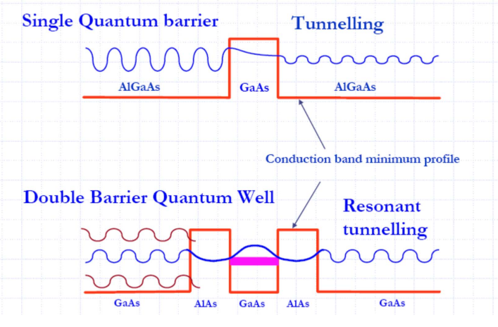
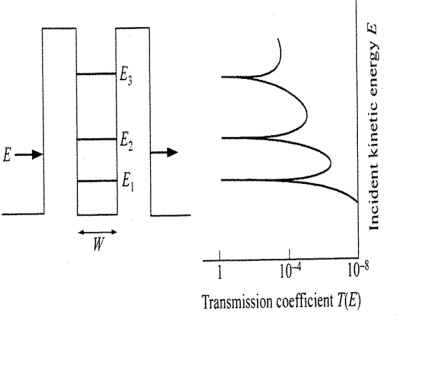
Resonant Tunneling